PlumSim

Interactive Gaussian plume visualizer for flares and stacks

PlumSim is a small, self-contained web tool that lets you explore how a gas plume from a flare or stack behaves in the atmosphere. It runs entirely in the browser, with no server or external dependencies, so you can keep a copy alongside design files and open it like a normal HTML page. The calculation engine is a steady-state Gaussian plume with a Briggs-style plume rise correction. It is meant as a fast, visual sketchpad to build intuition, compare cases, and sanity-check orders of magnitude, not as a replacement for PHAST or other validated dispersion codes.
The model represents a continuous release of a gas mixture from a vertical stack or flare. You enter the total mass rate of the mixture and the composition in percent for C1, C2, C3, C4, CO2, H2S, SO2 and H2O. You also choose which component you want to analyse as the “target species” by clicking the radio button next to it. PlumSim then computes the mass fraction of that species from the composition and multiplies it by the total mass rate to obtain the species mass rate that goes into the dispersion equations. In other words, if you double the H2S percentage while keeping total mass flow and all other conditions constant, the model will double the H2S concentrations everywhere.
For the dispersion itself, PlumSim uses a classic Gaussian plume expression at ground level. The ground concentration depends on the species mass rate, wind speed at stack height, crosswind and vertical dispersion coefficients (sigma_y and sigma_z), and the effective stack height. The code uses standard Pasquill–Gifford type correlations for sigma_y and sigma_z for stability classes A to F. Stability class is an explicit input, so you can explore how an unstable sunny day differs from a stable night. At each grid point on the map, the tool calculates the local x (downwind), y (crosswind) position relative to the source, evaluates sigma_y and sigma_z, applies the Gaussian formula, and then converts the resulting mass concentration in kg/m3 into ppmv using the target species molecular weight, ambient temperature, and ambient pressure via the ideal gas law.
Plume rise is handled using a simple Briggs-style approach that combines momentum and buoyancy effects. You supply the stack height, internal diameter, exit velocity and exit temperature, plus ambient temperature. From these, the code estimates a plume rise term based on exit momentum and on the buoyancy flux created by the temperature difference between the effluent and the ambient air. The effective stack height is the physical height plus this rise. A very hot, fast jet will get a larger effective height, which reduces ground-level concentrations near the source, while a cold, slow vent will remain closer to the physical stack height.
A basic building downwash correction is applied using the nearest building height input. If the effective height is lower than roughly three times the building height, the effective height is reduced toward about one and a half times the building height. This does not reproduce detailed wake effects but is a conservative nudge in the direction of higher ground concentrations when the stack is not clearly above local structures.
The tool is organized into several panels. In the Composition panel you choose a preset (Natural Gas flare gas, SRU Tail Gas, Acid Gas, or Custom), then refine the component percentages to match your case. The line at the bottom shows the total percentage so you can see how close you are to 100%. The text note area lets you store any comments, such as sample data or lab references. Below that, a small information line tells you which species is selected, the molecular weight used, its approximate share of the mixture, and the resulting species mass rate derived from the total mass rate.
The Release and Stack panel holds the core flow and geometry inputs. You enter total mass rate in kg/s, stack or flare height, internal diameter, exit velocity, exit temperature, wind speed at stack height, and stability class. The Environment and Site panel collects ambient temperature, ambient pressure, and nearest building height. The Contours panel defines the map size: maximum downwind distance and maximum crosswind distance on each side of the centerline. There is also a button to re-center the source handle on the canvas.
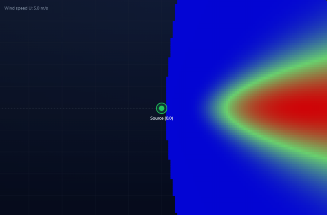
On the right side of the page you see the Contour Map. The source handle is a green ring located at the origin (0,0) of the coordinate system. You can drag this handle around if you later want to overlay the plume on other graphics; the underlying concentrations are always computed in coordinates relative to that point. The colors represent ground-level concentration of the selected species in ppmv. Blue is low, red is high. Below the map, a legend shows the color bar, the approximate minimum and maximum, and the calculated maximum concentration on the current domain. Colors are scaled relative to the maximum concentration for that run, so the pattern and extent are meaningful, but the brightness is normalized.
To run a simulation, follow this simple sequence. First, choose a composition preset that roughly matches your gas and adjust the component percentages. Second, choose the target species using the radio button and verify the molecular weight. Third, set total mass rate, stack height, diameter, velocity, exhaust temperature, wind speed and stability class. Fourth, enter ambient temperature, pressure and any relevant building height. Fifth, set the domain extents to cover the distances you care about. Finally, click the “Run model” button at the top right of the contour panel. The plume will be recomputed and the map updated. You can then hover the cursor over any point on the map to read x (downwind), y (crosswind), radial distance, and estimated concentration in ppmv at that point.
A Scenarios panel at the bottom of the left side lets you name, save, load and delete scenarios. The data is stored in the browser’s local storage only, so it does not leave your machine. This makes it easy to keep a small library of typical cases, such as “Main flare – normal”, “Main flare – windy”, or “SRU stack – cold start”.
Important limitations should always be kept in mind. PlumSim assumes a neutrally buoyant plume in the far field. It does not treat heavy gas behaviour, slumping, or pooling, which can be important for dense H2S and CO2 mixtures at low wind speeds and in stable conditions. It assumes steady-state, continuous release and flat terrain, with simple downwash. For design or regulatory work, PlumSim should be treated as a qualitative or screening tool only. Critical decisions, especially around toxic releases and exclusion zones, still need to be based on validated tools such as PHAST or ALOHA, or on detailed CFD and local standards. PlumSim is there to help you think, compare, and communicate, not to replace those tools.