BraySim

Interactive Brayton-cycle simulator with T–s diagram.

This project is a simple, educational gas turbine (Brayton cycle) simulator built entirely in HTML, CSS, and JavaScript with no backend. The goal is to help students “see” how basic thermodynamic inputs change the cycle on a temperature–entropy (T–s) diagram, using clean textbook assumptions rather than complicated real-world details. The interface is designed to be intuitive: a left-side control panel contains sliders for the main parameters, while the right side shows an interactive T–s plot that updates instantly as you adjust the controls. Below the chart, there are four compact text boxes used only to set the axis ranges (s min, s max, T min, T max), so you can zoom in or out for better understanding without changing the model itself.

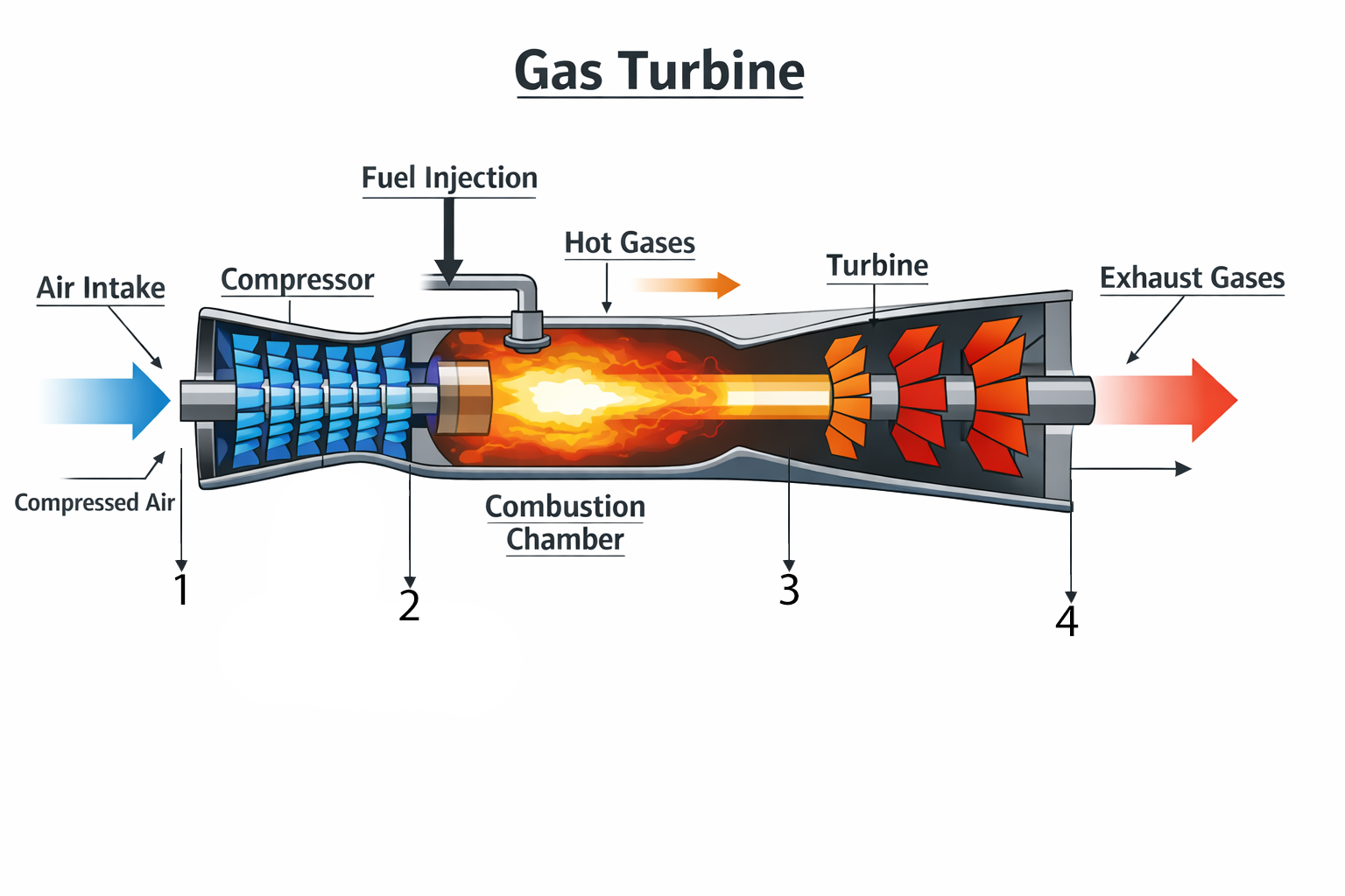
The simulator builds the cycle step-by-step using idealized processes. State 1 represents ambient inlet conditions. The user can set atmospheric pressure (P₁) and the compressor pressure ratio (PR = P₂/P₁). In the early ideal version, the compressor process (1→2) is isentropic, meaning entropy stays constant and the line appears vertical on the T–s diagram. The compressor outlet temperature increases according to the ideal-gas, constant-γ relationship, and the pressure at state 2 is simply P₂ = PR·P₁. In this educational model, intake pressure losses are ignored, so the compressor inlet pressure equals atmospheric pressure.

Next, the combustor (2→3) adds heat at constant pressure. Instead of modeling fuel flow or combustion chemistry, we use a simple temperature rise setting: ΔT = T₃ − T₂. This makes the combustor easy to understand: raising ΔT increases the peak cycle temperature T₃, the hottest point in the gas turbine. On a T–s diagram, constant-pressure heat addition is not a vertical line; entropy increases as temperature rises, so the curve bends to the right. In the simulator, that curve is drawn using the constant-pressure entropy relation for an ideal gas, which provides a smooth and realistic textbook shape without needing property tables.

Then the turbine expansion (3→4) produces work by expanding the hot gas back down to the inlet pressure. In our simple cycle, we assume the turbine exhaust pressure equals atmospheric pressure, so P₄ = P₁. Originally this expansion was also ideal (isentropic), creating another vertical line down on the T–s diagram. Finally, the cycle is closed by connecting state 4 back to state 1 with constant-pressure heat rejection (4→1) at P₁. This “closure” leg represents dumping heat to the surroundings and returning the working fluid back to inlet temperature, completing the Brayton loop in a clean, textbook way.

After the basic cycle is working, the simulator introduces a more realistic but still simple improvement: compressor and turbine isentropic efficiencies. These efficiencies show how real machines deviate from ideal behavior. The compressor efficiency (ηc) accounts for extra temperature rise required to achieve the same pressure ratio; lowering ηc increases T₂, which increases compressor work. The turbine efficiency (ηt) accounts for reduced work extraction compared to an ideal expansion; lowering ηt increases T₄, meaning the turbine leaves more energy in the exhaust. With these two sliders, students can immediately see the cycle “open up” on the T–s diagram: the compressor and turbine legs are no longer perfectly vertical, entropy increases across real components, and the net work shrinks.

To tie it all together, the simulator calculates and displays the overall thermal efficiency above the chart. Using a constant specific heat approximation, the compressor work is modeled as wc = cp(T₂ − T₁), the turbine work as wt = cp(T₃ − T₄), and the heat added in the combustor as Qin = cp(T₃ − T₂). The net work is wnet = wt − wc, and the thermal efficiency is ηth = wnet/Qin. This simple energy accounting matches the educational intent: it is fast, transparent, and easy for students to connect to the temperatures they see on the plot. The result is a compact learning tool that demonstrates the Brayton cycle visually, encourages exploration, and builds intuition about how pressure ratio, firing temperature, and component efficiencies influence performance.