AdsorbX

Fast 1D adsorption–regeneration bed simulator

PACKED-BED ADSORPTION + REGEN SIM (1D) — PROJECT NOTES (TXT FRIENDLY)
1) Purpose

We built a 1D packed-bed simulator for gas-phase adsorption + regeneration with:

Correct flow direction (up/down)

Adsorption/desorption kinetics (LDF)

3 axial layers (different properties per layer)

“Fast run” solving (run as fast as possible) + replay later

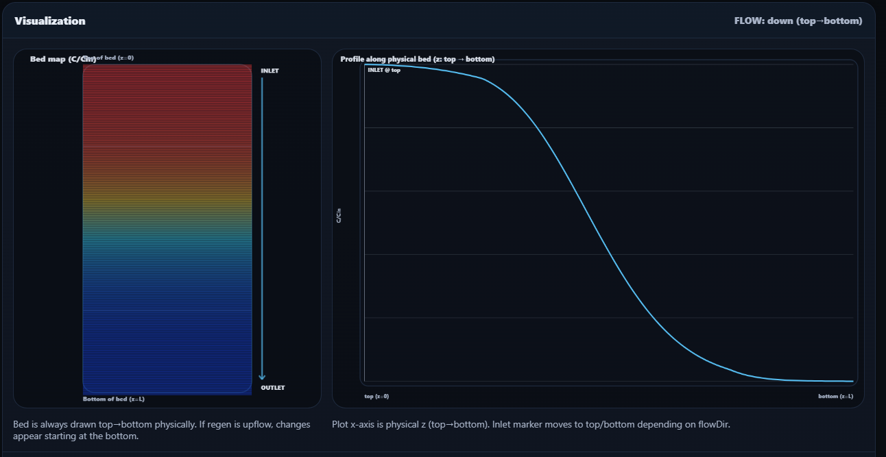
Visualization: bed colormap + concentration profile plot

Ability to chain adsorption -> regeneration using the ACTUAL bed state at the end of the previous run

This is NOT CFD.
It’s an engineering dynamic model for:

breakthrough behavior

regeneration effectiveness

front movement intuition

basic TSA/PSA-style cycle thinking

2) Modeling assumptions

2.1 One-dimensional approximation:

Ignore radial gradients

Bed is “uniform” radially

Properties vary only along the axial coordinate z

Coordinate system is PHYSICAL and FIXED:

z = 0 : top of bed

z = L : bottom of bed

IMPORTANT RULE:

The bed drawing does NOT flip when flow reverses.

Only the physics changes (inlet location, velocity sign, etc).

3) Governing physics

3.1 Gas-phase balance (per axial cell):
We use a standard 1D convection–dispersion balance with sink from adsorption:

eps * dC/dt = - u * dC/dz + Dax * d2C/dz2 - rhob * dq/dt

Where:

C = gas concentration (mol/m^3)

q = adsorbed loading (mol/kg)

eps = void fraction (-)

u = superficial velocity (m/s) SIGNED by flow direction

Dax = axial dispersion (m^2/s)

rhob = bulk density (kg/m^3)

3.2 Solid-phase kinetics (LDF):
dq/dt = kLDF * (qStar - q)

This is common/industry standard for packed-bed dynamics.

3.3 Equilibrium (linear isotherm + temperature effect):
qStar = K(T) * C

K(T) = Kref * exp( -alpha * (T - Tref) )

Meaning:

At higher T (regen), capacity drops (K smaller)

At lower T (ads), capacity increases (K larger)

4) Numerical implementation

4.1 Spatial discretization:

Bed is discretized into N ~ 140 axial cells

Uniform spacing: dz = L/(N-1)

Each cell stores:

C[i] (gas conc)

q[i] (solid loading)

4.2 Time integration:

Explicit time stepping

Convection: upwind differencing (depends on sign of u)

Dispersion: central differencing

LDF: explicit update

Time step dt is automatically chosen using stability limits:

convection (CFL)

diffusion number

LDF stiffness

We always pick the smallest safe dt.

5) Flow direction (CRITICAL)

We define flow direction with EXACT strings:

"down" = top -> bottom

"up" = bottom -> top

Bed coordinate never changes.

Implementation rules:
If flowDir = "down":

uSigned > 0

inletIndex = 0

outletIndex = N-1

If flowDir = "up":

uSigned < 0

inletIndex = N-1

outletIndex = 0

Why this matters:

Convection term uses uSigned

Inlet boundary condition depends on inletIndex

During regeneration with upflow, the desorption front must move upward physically

Important design choice:

We refused “visual hacks” like flipping arrays or just swapping labels.

The simulation and visualization must represent the same physical bed.

6) Boundary conditions

Inlet (Dirichlet):

C[inletIndex] = Cin

Outlet (approx Neumann / zero-gradient):

C[outletIndex] = C[neighbor]

Cin comes from converting ppmv to mol/m^3 via ideal gas:

Ctot = P/(R*T)

Cin = Ctot * (ppmv * 1e-6)

7) 3-layer adsorbent bed

The bed is divided into 3 axial sections (L1, L2, L3).
Each layer has different:

Kref (equilibrium strength)

kLDF (kinetics)

Layer assignment is by z position (physical), not by “flow direction”.
That allows guard beds / polishing beds / mixed media.

8) Adsorption vs regeneration

Adsorption run (typical):

higher inlet ppmv

lower temperature

often downflow

bed loads up (q increases)

Regeneration run (typical):

purge ppmv ~ 0 (or low)

higher temperature

often upflow

bed unloads (q decreases)

9) Bed state continuity (very important)

Principle:

Regeneration must run on the CURRENT bed condition if it exists.

No “reset” unless user explicitly chooses it.

Implementation:
After any run finishes:
currentBed = {
C(z) array,
q(z) array,
timestamp,
note
}

Next runs can start from:

Initial Bed State (user-defined)
OR

Current Bed State (from last run)

This enables:

realistic cycles

partial regenerations

operator-like workflow

10) Fast-run + replay philosophy

Real-time solving + drawing is slow and CPU heavy.
So we separate:

Solve fast (no drawing, no DOM updates)

Save snapshots (time series of C profiles)

Replay later with:

play/pause

speed control

time slider

This is how many process simulators feel: solve first, inspect later.

11) Visualization rules

Physical bed view:

index i=0 is always top on screen

index i=N-1 always bottom on screen

NO flipping of the colormap

What changes when flow reverses:

inlet/outlet marker positions

flow arrow direction

which end is the boundary condition

which end is reported as “outlet”

So if regen is upflow:

you should see changes start at the bottom and move upward (physically)

12) What this model IS / IS NOT

IS:

1D dynamic packed-bed model (convection + dispersion + LDF)

Good for breakthrough/regeneration intuition

Layered bed support

Honest and consistent flow direction behavior

IS NOT:

CFD

vendor design tool

full thermal TSA with energy balance (not yet)

multi-component competitive adsorption (not yet)

pressure drop model (not yet)

13) Why the architecture matters

We intentionally kept it:

transparent

debuggable

extendable

Future add-ons (easy to plug in):

energy balance / thermal front

multicomponent adsorption

pressure drop (Ergun)

multi-cycle convergence to cyclic steady state

time-varying boundary conditions (ramps, steps)

14) Key lesson from debugging

The main bug class we fought was:
“solver is correct but visualization flips the bed / labels”

Final rule:

No visual tricks.

Physical coordinate system stays fixed.

Flow direction is handled in the math via signed velocity + inlet index.